Thursday, September 4, 2014

Collecting Camera (EXIF) Data through R

Slowly, but surely, I'm working on a way to organize all my photos on the various folders on my computer.  It's a mess.  I've got folders with thousands of pictures, copies of folders, files with different names, etc.

I've been trying to come up with a way to create a nice, organized folder with only one copy of each of my photos with them all organized into subfolders.  It's tricky, though, because I don't really know what I have.

Enter EXIF data.  This is data that the camera applies to each file it creates when it captures a photo.  There's potentially a lot of data available, but it depends on the camera manufacturer.  This can include the photos creation date, the dimensions of the photo, the camera make and model, and gps data, such as latitude, longitude and altitude.

There's supposedly a unique ID value cameras can assign, which is supposed to be globally unique.  Unfortunately, most of the pictures I took didn't have that available.  However, there's plenty of other data that I can combine to check for uniqueness.

There's this great, free tool that you can use to read EXIF data.  You use the tool through a command prompt window.  This really works great since you can interact with a command prompt window using R.

Building on what I learned from this blog post, I built a function that I can utilize to go through a bunch of my photo files.  It's pretty basic.

#This function calls exiftool, a command line application that returns exif data from photo files, searches the file for pertinent data, and returns those values in a

#vector.  If nothing is found, ‘UNKNOWN’ is returned.


getexifdata <- function(filename){

cmd <- paste('exiftool -c ' ,shQuote('%.6f'), shQuote(filename)) #create the MSDOS command we’ll be using.

exifdata <-  system(cmd,intern=T)  #use the MSDOS command using the system function.


#the system command that calls exiftool returns a vector.  Each line consists of one property value of the photo.  It’s starts with the name of the property and the actual value starts at the 35th character.

#these next few lines are searching the returned vector for specific property value using the name found at the beginning.  

#If found, collect the property value starting at character 35.  Since there can be multiple matches, collect only the first item found. Search different possible labels as camera companies name stuff differently.


imageheight <- substring(exifdata [grep('^Exif Image Height        |Image Height  ',exifdata )[1]],35,nchar(exifdata [grep('^Exif Image Height       |Image Height  ',exifdata )[1]]))

imagewidth <- substring(exifdata [grep('^Exif Image Width      |Image Width ',exifdata )[1]],35,nchar(exifdata [grep('^Exif Image Width      |Image Width ',exifdata )[1]]))

gpslatitude <- substring(exifdata [grep('^GPS Latitude      ',exifdata )[1]],35,nchar(exifdata [grep('^GPS Latitude       ',exifdata )[1]]))

gpslongitude <- substring(exifdata [grep('^GPS Longitude      ',exifdata )[1]],35,nchar(exifdata [grep('^GPS Longitude       ',exifdata )[1]]))

cameramodel <- substring(exifdata [grep('^Camera Model Name      ',exifdata )[1]],35,nchar(exifdata [grep('^Camera Model Name       ',exifdata )[1]]))

createdate <- substring(exifdata [grep('^Create Date      |File Creation Date',exifdata )[1]],35,nchar(exifdata [grep('^Create Date      |File Creation Date',exifdata )[1]]))


#If no value is found, NA is returned. Set to ‘UNKNOWN’


if (is.na(imagewidth)){imagewidth <- 'UNKNOWN'}

if (is.na(imageheight)){imageheight <- 'UNKNOWN'}

if (is.na(gpslatitude)){gpslatitude <- 'UNKNOWN'}

if (is.na(gpslongitude)){gpslongitude <- 'UNKNOWN'}

if (is.na(cameramodel)){cameramodel <- 'UNKNOWN'}

if (is.na(createdate)){createdate <- 'UNKNOWN'}

#return values as a vector.

return(c(imagewidth,imageheight, gpslatitude, gpslongitude,cameramodel, createdate))


}


NOTE: Your mileage may definitely vary on this one.  Camera models assign labels for their data differently.  If you're like me and you have pictures in your folders from lots of different camera manufacturers, you've got to take that into account and change the labels you are looking for. Some also put in their EXIF data values that others don't.

Another good place to get data on photo files is with the file.info function.  I talk about that here.

Wednesday, July 16, 2014

Get a custom file list with R

I'm working on a way to better manage my files on my computer.  I've got tons of duplicate photos and mp3s that I've copied to remote drives.  Additionally, I've got folders with hundreds of poorly named files.  Opening one of these folders is a nightmare if I happen to open one with a thumbnail view!

Because I've been playing around with it recently, I thought I would see what R could do to help me.  I've got a ways to go, but it looks like R has a great function that can put the specifics of a file within a data set, file.info.

file.info("C:\\users\\doug shartzer\\messy folder\\song1.mp3")

Additionally, you can provide file.info with more than one file at a time within a vector.  In fact, you can pass it an entire folder using the dir function on a folder, which will create a vector containing all the files within the provided folder.  Be sure to use the full.names argument on the dir function to get the full path, which file.info needs.

file.info(dir("c:\\users\\doug shartzer\\messy folder\\",full.names=T))

What's even better?  You can provide the dir function with a vector of folder names to get a giant dataset of file details with just one line of code.  It also has a recursive argument that'll include files within each folder's subfolder.  

file.info(dir(c("c:\\","d:\\","e:\\"), full.names=T, recursive=T)

Lastly, dir also allows you to limit your list further by accepting regular expressions in its pattern argument to limit the list of files returned. I can limit my list of files to just pictures and music files. 

 file.info(dir(c('c:\\','d:\\','e:\\'),recursive=T,full.names=T,pattern='+mpg$|+mp3$|+jpg$'))

So, building a list of the files I've got to go through appears to be a breeze!  Now I've got to figure out where to go from here...


Monday, March 17, 2014

Getting a sample from a large data file with R

I'm working on a little project to attempt to cluster the voters in North Carolina into congressional districts.  My goal is to see if there's a way to have a computer draw the districts instead of relying on people with potential biases.

I quickly ran into quite a big wall when I reviewed the file listing all the voters in North Carolina.  I should have suspected that it would be huge!  A file consisting of around 7.5 million voters (both active and invalid) and around 60 columns is about 4.5 gigabytes.  Considering I have 4 gigabytes of RAM, I needed an alternative plan.

Well, I know that I just wanted a sample of this file.  I'm going to try and geocode these addresses and use the lat/long coordinates for the clustering.  As I've stated in previous posts, geocoding has daily limits. Geocoding tons of addresses can take serious time.

I didn't have too much success using the standard read.table function in R.  There are skip and nrow parameters, but they didn't seem to help too much when dealing with my RAM woes.  I also tried the Fread package, but my data had some flaws and Fread wasn't too flexible working around it.

I took a really simplistic approach to my problem by utilizing the lowly file command that comes standard with R.  First, a loop with the file command went through each line and copied only rows that didn't have problems.  In my situation, there were extra quote symbols in some of the lines. Those lines weren't worth it.  So, I skipped them.

 I also took out voters that weren't listed as ACTIVE or INACTIVE.

v <- file("c:\\users\\doug shartzer\\documents\\data\\ncvoter_Statewide.txt")

open(v)

while(length(line <- readLines(v,1)) > 0) {

if (sum(table(strsplit(line,'"'))) == 140) {

if (strsplit(line,'"')[[1]][[10]] == 'ACTIVE' | strsplit(line,'"')[[1]][[10]] == 'INACTIVE' ) {

write(line, 'c:\\users\\doug shartzer\\documents\\data\\voter_good_all.txt',append=T)

}

}

if (sum(table(strsplit(line,'"'))) != 140) {

print(line)

}

}

close(v)

q()


Although it did take a while to run (16 hours), I didn't run into any problems with memory.

After that, I collected a sample and wrote those voters to another file.

s <- sample(7500000, 75000)

v <- file("c:\\users\\doug shartzer\\documents\\data\\voter_good_all.txt")

open(v)

while(length(line <- readLines(v,1)) > 0) {

if (x %in% s){

write(line, 'c:\\users\\doug shartzer\\documents\\data\\voter_sample_03142014.txt',append=T)

}

}

shartzer\\documents\\data\\voter_run_status.txt',append=T)

close(v)


q()

After this process, I had a much more manageable file to play around with.

Wednesday, December 18, 2013

Getting an Antenna Pointing in the Right Direction for an HDHomerun Tuner

Getting your antenna pointed in the right direction for a Silicon Dust HDHomerun tuner isn't too big of a chore if you have an Android phone and a little patience.

I'm assuming you have an HDHomerun tuner plugged into your network.

First, figure out what kind of antenna you need.  AntennaWeb is a great resource for this. Provide your street address and zip code and it'll tell you how far away TV stations are from your house and which direction you need to point your antenna.


I went a little overkill and bough the DB4e antenna from Antenna's Direct.  

Next, figure out how you'll mount your antenna.  For me, I found a broken shower curtain rod that I used for a mounting pole in a scrap piece of lumber.  I then attached the scrap piece to the joists in the attic.  

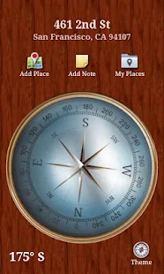
Using the degree values from AntennaWeb, point your antenna in the right direction.  There's a great free Compass app available in the Android store. Point the top of your phone in a direction and it'll tell you which direction in degrees you are pointing in the bottom left corner.    
.


Use the HDHomeRun Setup application on your computer to scan for channels.  This can be found under the Digital Antenna tab.  After you hit scan, you'll see all the channels your antenna can tune.


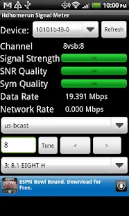
To watch a channel, click on one of the hyperlinks.  If the quality is less than desired, adjust the antenna.  If the antenna is far away from your computer (like mine), there's another awesome free Android app that can check signal strength:  HDHomerun Signal Strength.


Hopefully, with just a couple of adjustments using the Compass and Signal Strength apps, you'll reach optimal tuning.  This was a big help for me and my antenna mount in the attic.  Here it is after just an hour or so of mounting and adjusting.  


Monday, November 11, 2013

Random Maps of Wake County Demographics

I've been playing around a lot with mapping data recently.  Here are some maps that represent voters in Wake County, North Carolina.  Each map represents a sample of 35000 voters collected from the North Carolina State Board of Elections in October 2013.  Each dot is a single voter and their residential location.


My data was collected from the following sources:

Voter registration information from the NC Board of Elections:  ftp://www.app.sboe.state.nc.us/
Mapping shapefiles from Wake county:  http://www.wakegov.com/gis/services/pages/data.aspx

Geocoding the addresses was done by Texas A&M's Geoservices:  http://geoservices.tamu.edu/

Sunday, November 10, 2013

A Map of Registered Republicans and Democrats in Wake County


Here's my R code.  I utilized the R rgdal package for creating the maps.
This assumes that you've already got your voter data loaded into R.

roads <- readOGR("c:\\data\\poly\\wake_streets\\streets.shp","streets")
roadmap <- spTransform(roads, CRS("+proj=longlat +datum=WGS84"))
county <- readOGR("C:\\data\\poly\\nc_counties\\NC_State_County_Boundary_NAD83HARN.shp",'NC_State_County_Boundary_NAD83HARN')
countymap <- spTransform(county, CRS("+proj=longlat +datum=WGS84"))

plot(roadmap[roadmap$CLASSNAME == 'INT',],col='black',border='black', lwd=.5,axes=F,xlim=c(-79,-78.2),ylim=c(35.5,36.1))
plot(countymap[countymap$County == 'Wake',], add=T)
plot(roadmap[roadmap$CLASSNAME == 'USHWY',],col='black',border='black', lwd=.5, add=T)
points(vtx[vtx$party == 'REP','lng'],vtx[vtx$party == 'REP','lat'],col = rgb(255,0,0,50,maxColorValue=255),cex=.2,pch=20)
points(vtx[vtx$party == 'DEM','lng'],vtx[vtx$party == 'DEM','lat'],col = rgb(0,0,255,50,maxColorValue=255),cex=.2,pch=20)
title("Registered Wake County Republican or Democrats \n (sample of 35,000) - Oct 2013")

My data was collected from the following sources:
Voter registration information from the NC Board of Elections:  ftp://www.app.sboe.state.nc.us/
Mapping shapefiles from Wake county:  http://www.wakegov.com/gis/services/pages/data.aspx

Geocoding the addresses was done by Texas A&M's Geoservices:  http://geoservices.tamu.edu/


Friday, November 1, 2013

Do Running Backs Drafted in Earlier Rounds Perform Better in the NFL?

It appears there is a decent correlation  (0.5, according to my calculations) between an NFL running back's performance and their their draft position.  I'm measuring performance using their career yard total.

This data does NOT include yardage for the 2013 season or players drafted in 2013.